Part 2: Designing an Edge AI Vision Classifier for Farm Security

14-Hour Runs, Overfitting Battles, and Hitting the Resolution Wall. Squeezing every drop of performance out of CIFAR-10 with advanced regularization and 14-hour hyperparameter sweeps.

Pulling Out All the Regularization Stops

Following our baseline model's struggle with overfitting, we knew we had to introduce advanced architectural layers and training strategies to force our network to generalize. We upgraded our data pipeline and training loop with three powerful weapons:

1. Transfer Learning with MobileNetV2

Instead of training all features from scratch, we imported MobileNetV2—a highly efficient network pre-trained on millions of high-resolution ImageNet photos. We froze its base layers to preserve its robust, pre-learned edge-detection capabilities, appending our custom classification head on top. This dramatically reduced the number of trainable parameters while giving us access to elite spatial feature extractors.

2. Dropout and Early Stopping

To prevent individual neurons from co-adapting and memorizing training patterns, we integrated Dropout layers to randomly deactivate 40% of our hidden units on every forward pass. We also implemented an EarlyStopping callback. This acted as our autopilot, monitoring our validation loss and automatically halting training when performance plateaued, preventing the model from over-optimizing.

early_stopping = tf.keras.callbacks.EarlyStopping(
    monitor='val_loss', 
    patience=5, 
    restore_best_weights=True
)

3. CutMix Data Augmentation

To push generalization to the absolute limit, we implemented CutMix. During training, CutMix programmatically cuts a rectangular patch from one training image (e.g., a car) and pastes it onto another (e.g., a horse), blending their labels proportionally. This forces the network to classify images based on partial visual cues rather than relying on a single, easy-to-spot feature.

The 14-Hour Optimization Sweep

To find the absolute sweet spot for our hyperparameters, we set up an extensive, automated search. We utilized Bayesian Optimization to sweep through various configurations of learning rates, weight decay schedules (using the AdamW optimizer), and spatial dropout rates.

Because we committed to running this on consumer-grade local hardware, this sweep was an absolute endurance test—our systems ran hot for over 14 hours straight overnight.

The Breakout Metric... and the Disturbing Truth

When we analyzed the final run, our optimization had worked incredibly well. Our optimized network (Model 2) achieved a validation accuracy of 72.67%—representing a massive 10.5% improvement over our simple baseline model.

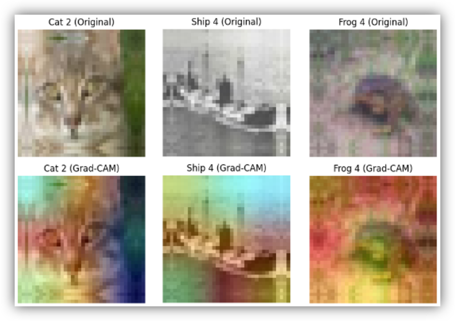
I couldn’t rely on accuracy alone. I generated a multiclass confusion matrix and used Grad-CAM (Gradient-weighted Class Activation Mapping) to produce visual heatmaps of the model’s decision-making process.

Our model had a remarkably high success rate at identifying "Frogs." But the Grad-CAM heatmaps revealed that the model was cheating.

Because frogs in our dataset were almost always photographed sitting on lush green grass, our network had learned a shortcut: "If there is a lot of green grass, predict Frog." This is known as Shortcut Learning. The model hadn't actually learned what a frog looked like; it had merely learned to detect green backgrounds. If we deployed this prototype around our farm, it would label a green truck or lawnmower as a "frog" with 99% confidence.

Hitting the Physical Wall

We realized we had hit a physical limitation. At 32x32 pixels, the target objects themselves were simply too small and blurry for the network to extract high-fidelity spatial details without relying on background context.

If we wanted a robust, trustworthy vision system for real-world farm monitoring, we had to make an executive architectural decision: We had to pivot.

We decided to upgrade our system to the STL-10 dataset. STL-10 is specifically designed for evaluating unsupervised and semi-supervised learning. Most importantly:

• Resolution: It increases image size from 32x32 to 96x96 pixels—representing a 9-fold increase in total pixel density.
• The Class Trade-off: To transition datasets, we had to swap out a few target categories. We lost Frogs and Automobiles, but gained Monkeys and Cars.

For a farm-security and observation system, losing frogs while maintaining a massive leap in object resolution was a trade-off we were more than willing to make. In Part 3, we’ll look at how we applied every lesson learned from our sandbox phase to build an elite, 96x96 deployment-ready model.

• 👾 Test the live application: View on Hugging Face
• 💻 View the production codebase: View on Github

📝 Author's Note & Original Files

This blog series is adapted from an academic instructional design project completed during my university coursework. It is an AI-generated summary (until I get a chance to rewrite it, then I will remove this note). The original goal was to break down complex machine learning architectures into digestible lessons for beginners.

If you are an educator, student, or just curious to see the original academic formatting, you can download the raw instructional draft here: