Part 3: Designing an Edge AI Vision Classifier for Farm Security
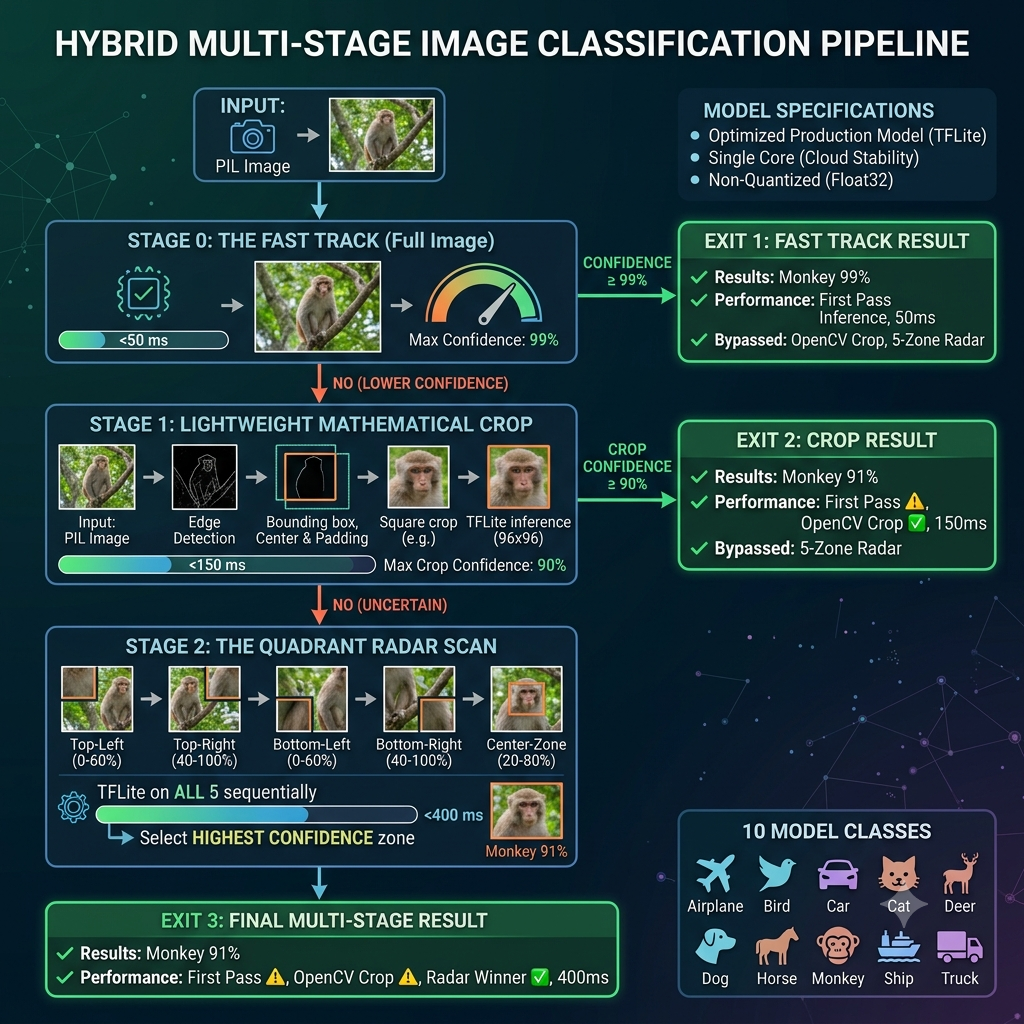
Building our high-resolution champion model, compressing it into TFLite, and writing a robust Gradio app with a 3-tier sequential inference pipeline.
Rebuilding for 96x96 Resolution
Armed with the hard-won lessons from our CIFAR-10 sandbox phase, we moved rapidly with STL-10. Because we were now processing 96x96 images, we knew we couldn't start from scratch. We set up a rapid prototyping environment to evaluate three pre-trained, lightweight backbones: ResNet50V2, EfficientNetB0, and MobileNetV2.
To keep our development cycle highly efficient and avoid repeating our 14-hour overnight wait, we implemented a "Debug Mode" flag in our training scripts.
When active, this flag bypassed heavy data augmentations and restricted our training to a tiny, fractioned subset of the data for a single epoch. This let us verify that our inputs, outputs, tensor shapes, and loss calculations were 100% correct in less than 60 seconds before committing to full training runs.
Our rapid testing paid off. We selected MobileNetV2 as our backbone for its incredible balance of spatial feature extraction and rapid edge inference speed.
The Champion Model Results
By applying our optimized pipelines—CutMix, early stopping, and fine-tuning our pre-trained backbone—our STL-10 champion model shattered our previous records.
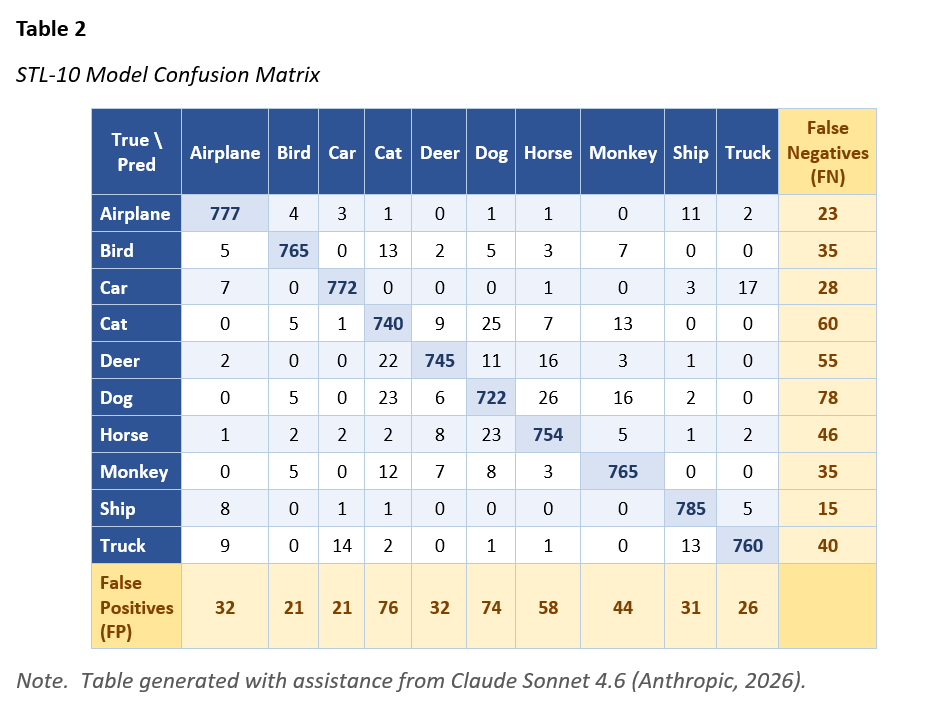
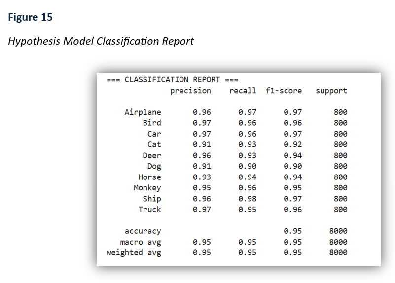
We achieved F1-scores of 90% or higher across almost all ten classes. More importantly, our Grad-CAM checks confirmed that the model was now focusing directly on the actual structural boundaries of the vehicles and animals themselves, rather than cheating on background textures.
Transitioning to the Edge: Exporting to TFLite
To make this model run locally on cheap, consumer-grade hardware (like a Raspberry Pi or an old office computer acting as a central farm hub), we couldn't deploy our bulky, uncompressed Keras weights.
We exported our trained model and converted it into a TensorFlow Lite (TFLite) format. This step stripped away unnecessary training metadata and structured the mathematical weights for highly efficient, single-core local CPU execution.
Architecting the 3-Tier Sequential Inference Pipeline
For our final user-facing deployment, we built an interactive web application using Gradio on Hugging Face. However, we didn’t want to just pass images directly to the model. In a real farm setup, objects of interest might be far away, small, or hidden in a corner of the frame.
To solve this, we engineered a custom, 3-Tier Escalation Pipeline in Python:
Stage 0: The Fast Track (Full Image)
First, we run inference on the raw, full-sized image. If the model is exceptionally confident (confidence score ≥ 99%), we bypass all other logic. This ensures that close-up, obvious subjects are processed in milliseconds with zero CPU overhead.
Stage 1: The Smart Crop (OpenCV Canny & Laplacian)
If the first pass is uncertain, we escalate. We use classical computer vision (OpenCV Canny Edge Detection and a Gaussian Blur) to find the dense boundaries of visual interest within the frame. We automatically draw a padded bounding box around the densest edge clusters, crop the image to focus on that subject, and run inference on the crop. If this crop confidence is ≥ 90%, we output the result.
Stage 2: The Quadrant Radar Sweep
If both the full image and smart crop fail to yield a highly confident answer, we run our final fallback: a 5-Zone Quadrant Sweep.
We programmatically slice the image into five overlapping regions (Top-Left, Top-Right, Bottom-Left, Bottom-Right, and Center-Zone) and run a rapid sequential inference sweep across all five zones. The app compiles the results, identifies which quadrant yielded the highest confidence score, and returns that prediction as the winning classification.
The Code: Our Gradio Application
Here is the core logic of our localized edge application. This code is deployed live and demonstrates the complete hybrid OpenCV/TFLite escalation pipeline:
# Stage 1: OpenCV Smart Edge Cropper
def traditional_smart_crop(pil_image):
    # Convert PIL to OpenCV format
    img_cv = cv2.cvtColor(np.array(pil_image), cv2.COLOR_RGB2BGR)
    gray = cv2.cvtColor(img_cv, cv2.COLOR_BGR2GRAY)
    blurred = cv2.GaussianBlur(gray, (5, 5), 0)
    edges = cv2.Canny(blurred, 50, 150)

    # Find coordinates of all edge pixels
    pts = np.argwhere(edges > 0)
    if len(pts) == 0:
        return pil_image

    y_min, x_min = pts.min(axis=0)
    y_max, x_max = pts.max(axis=0)

    h, w = gray.shape
    pad_x, pad_y = int((x_max - x_min) * 0.15), int((y_max - y_min) * 0.15)

    left, top = max(0, x_min - pad_x), max(0, y_min - pad_y)
    right, bottom = min(w, x_max + pad_x), min(h, y_max + pad_y)

    # Convert crop boundaries to a perfect square
    side = max(right - left, bottom - top)
    center_x, center_y = left + ((right - left) / 2), top + ((bottom - top) / 2)

    left, top = max(0, int(center_x - side / 2)), max(0, int(center_y - side / 2))
    right, bottom = min(w, int(center_x + side / 2)), min(h, int(center_y + side / 2))

    # Safety guardrail: abort crop if math yields invalid dimensions
    if right - left < 10 or bottom - top < 10:
        return pil_image

return pil_image.crop((left, top, right, bottom))- 👾 Test the live application: View on Hugging Face
- 💻 View the production codebase: View on Github
📝 Author's Note & Original Files
This blog series is adapted from an academic instructional design project completed during my university coursework. It is an AI-generated summary (until I get a chance to rewrite it, then I will remove this note). The original goal was to break down complex machine learning architectures into digestible lessons for beginners.
If you are an educator, student, or just curious to see the original academic formatting, you can download the raw instructional draft here: