By William M — Jul 16, 2026

Part 1: Designing an Edge AI Vision Classifier for Farm Security

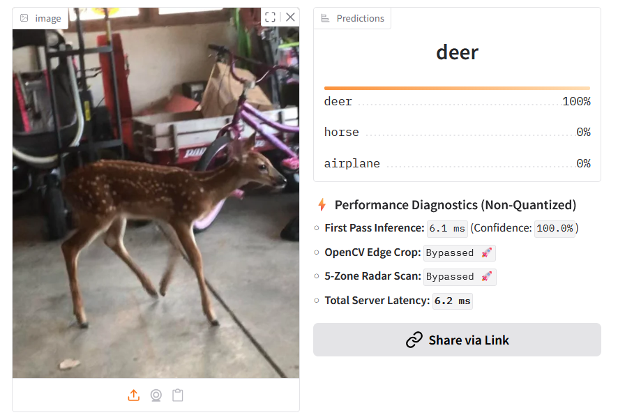
The Mission: Off-Grid, Local-First Farm Intelligence

Imagine you have an off-grid agricultural facility. You’ve got perimeter security cameras, a driveway sensor, and maybe even a pre-programmed automated drone patrolling the fence lines. You want to automatically identify vehicles, incoming aircraft, livestock, and local wildlife to trigger automated alerts.

But there is a catch: the facility is off-grid. You cannot rely on high-bandwidth satellite internet or expensive cloud APIs like AWS or Google Cloud. The system must process video stills locally, on consumer-grade hardware, without an active internet connection.

In our machine learning curriculum, my cohort took on this challenge. We wanted to build a localized edge prototype capable of classifying ten critical environmental categories:

Vehicles/Transit: Airplanes, Automobiles, Trucks, Ships
Animals/Wildlife: Birds, Cats, Deer, Dogs, Frogs, Horses

To keep our initial development fast and highly iterative, we began our journey in a sandbox environment using the classic CIFAR-10 dataset—a balanced benchmark of 60,000 32x32 pixel images representing these exact ten categories.

Step 1: Preprocessing & Safeguarding the Data Pipeline

Before a single tensor was passed to a neural network, we had to address an essential truth of machine learning: Real-world data is messy. Even when utilizing a curated benchmark like CIFAR-10, building a production-grade pipeline means establishing programmatic gatekeepers.

1. Programmatic Blur Filtering

Low-quality, heavily blurred images degrade a model’s ability to learn distinct edge features. We built an automated blur-detection gatekeeper utilizing OpenCV to calculate the Laplacian variance of incoming images.

If the variance fell below a conservative threshold of 10.0, the image was flagged as too blurry and discarded from our pipeline, ensuring the model only trained on structured visual data.

import cv2
import numpy as np

def detect_blur(image_path, threshold=10.0):
    # Load image in grayscale
    image = cv2.imread(image_path, cv2.IMREAD_GRAYSCALE)
    # Compute the Laplacian (second derivative) and return its variance
    laplacian_var = cv2.Laplacian(image, cv2.CV_64F).var()
    
    if laplacian_var < threshold:
        print(f"Skipping {image_path}: Image is too blurry ({laplacian_var:.2f})")
        return False
    return True

2. The Poison of NaN Values

We also programmed safety checks to scan for corrupted pixel values, specifically NaN (Not a Number) or infinite values. In deep learning, a single NaN pixel is toxic. Because of how backpropagation works, that single NaN value will multiply across weight matrices and activation functions during training. Within a few steps, the entire network's weights will degrade into an untrainable block of NaNs—a silent killer of training runs.

3. Injecting Synthetic Noise for Generalization

Intuitively, you might think we should smooth out noisy images before training. However, we chose a counterintuitive but highly effective strategy: we intentionally injected synthetic noise into our training data.

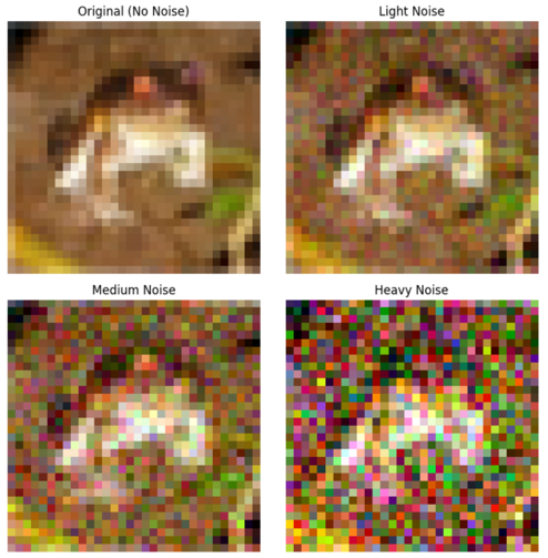
By augmenting our training set with noise, we forced our Convolutional Neural Network (CNN) to ignore micro-level pixel textures and focus on macro-level shapes and structural boundaries. This significantly boosted the model's eventual generalization to unpredictable, real-world outdoor lighting.

Step 2: Formulating Categorical Targets

To classify ten unique, non-ordered categories (e.g., a "cat" is not numerically "greater than" a "frog"), we transformed our integer class labels (0 through 9) into One-Hot Encoded vectors.

If we kept the labels as raw integers, the neural network’s loss function would treat the classes as a continuous scale. It would assume that predicting a "car" (class 2) for a "cat" (class 3) is a minor, acceptable error, while predicting a "truck" (class 9) is a massive failure. By converting class labels to 10-dimensional binary vectors, we ensured that every incorrect prediction was penalized equally.

Step 3: Building the Baseline Model

With our data pipeline sanitized and targets one-hot encoded, we constructed Model 1: The Baseline CNN using Keras and TensorFlow.

We kept the architecture classic and lightweight, utilizing alternating blocks of Conv2D layers (to extract local spatial features), BatchNormalization (for training stability), and MaxPooling2D (to reduce dimensionality and introduce translation invariance). We finished the network with a Dense block mapping to a 10-unit Softmax output layer to calculate the probability distribution across our classes.

import tensorflow as tf
from tensorflow.keras import layers, models

def build_baseline_cnn(input_shape=(32, 32, 3), num_classes=10):
    model = models.Sequential([
        # Block 1
        layers.Conv2D(32, (3, 3), activation='relu', padding='same', input_shape=input_shape),
        layers.BatchNormalization(),
        layers.MaxPooling2D((2, 2)),
        
        # Block 2
        layers.Conv2D(64, (3, 3), activation='relu', padding='same'),
        layers.BatchNormalization(),
        layers.MaxPooling2D((2, 2)),
        
        # Classification Head
        layers.Flatten(),
        layers.Dense(128, activation='relu'),
        layers.Dropout(0.3),
        layers.Dense(num_classes, activation='softmax')
    ])
    return model

The Result: High Training, Poor Validation

Our baseline model compiled effortlessly and trained incredibly fast. However, when we plotted our training curves, the classic deep learning trap stood revealed: Overfitting. While our training accuracy steadily climbed past 85%, our validation accuracy stalled in the mid-60s. The model was simply memorizing our training dataset's specific pixel layouts rather than learning true, generalizable concepts.

More importantly, looking at the 32x32 images, we realized we were fighting an uphill battle. At 32x32, a distant deer or automobile is represented by just a tiny handful of pixels.

Determined to break through this performance ceiling, our class geared up for a massive battle against overfitting—a battle that would push our consumer hardware to its limits, which we will dive into in Part 2.

👾 Test the live application: View on Hugging Face
💻 View the production codebase: View on Github

📝 Author's Note & Original Files

This blog series is adapted from an academic instructional design project completed during my university coursework. It is an AI-generated summary (until I get a chance to rewrite it, then I will remove this note). The original goal was to break down complex machine learning architectures into digestible lessons for beginners.

If you are an educator, student, or just curious to see the original academic formatting, you can download the raw instructional draft here: