Data Analytics Capstone - Code Reference

#Cell 1
#Import the packages required to complete the test.

#Pandas is imported to deal with tabular data.
import pandas as pd
#Numpy is imported to deal with mathematical functions.
import numpy as np
#Missingno is imported to deal with nulls.
import missingno as msno
#Pyplot and Seaborn are imported to deal with visualizations.
import matplotlib.pyplot as plt
import seaborn as sns
#Math is imported as it will help with capping outliers
import math
#Stats is imported for running the t-test.
import scipy.stats as stats
#For formatting list output in a more readable format
from pprint import pprint

#Warnings is used to supress messages about future version deprecation.
import warnings
warnings.simplefilter(action='ignore', category=FutureWarning)


#Import data from data set files.

scores = pd.read_csv ('C:\\Users\\will\\Desktop\\Courses\\11 - Capstone - D214\\Task 2\\Data\\scores.csv',
                 index_col=0)

free_lunch_percentages = pd.read_csv \
('C:\\Users\\will\\Desktop\\Courses\\11 - Capstone - D214\\Task 2\\Data\\free_lunch_percentages.csv', index_col=0)


#Converting all null value representations to 'nan'
#"free_lunch_percentages" has nulls reported as '#NULL!'.  Changing '#NULL!' to 'nan' with replace() method (Inada, n.d.).
free_lunch_percentages.replace("#NULL!", np.nan, inplace=True)
#"scores" has nulls reported as '#NULL!'.  Changing '-' to 'nan' with replace() method (citation).
scores.replace("-", np.nan, inplace=True)


#Only include relevant variables
dependent = scores[["Division Name","School Name","English_2015_16","Mathematics_2015_16","History_2015_16","Science_2015_16"]]
independent = free_lunch_percentages[["free_per_1516"]]


#Output basic statistics on each dataframe.
print("\n")
print("Dependent data frame statistics")
print(dependent.describe())
print("\n")
print("Independent data frame statistics")
print(independent.describe())
Dependent data frame statistics
Division Name School Name English_2015_16 \
count 1822 1831 1813
unique 132 1758 64
top Fairfax County Mountain View Elementary 85
freq 192 6 89
Mathematics_2015_16 History_2015_16 Science_2015_16
count 1814 1768 1750
unique 62 49 71
top 90 94 83
freq 95 99 79
Independent data frame statistics
free_per_1516
count 1910
unique 1610
top 100.00%
freq 60
#Cell 2
#Join data on both dataframes using join() method (Bobbit, 2021).
df = dependent.join(independent)
#Define function to count nulls and output counts/percentage
def nullcounter(dataframename):
print("\n Your null count for \"{dname}\" is: \n".format(dname=dataframename))
run = '''nullcounter = pd.DataFrame(({name}.isna().sum()), columns=["Null Count"])
nullcounterpercent = pd.DataFrame(({name}.isna().mean() *100), columns=["Null Count"])
nullcounter['Null %'] = nullcounterpercent
print(nullcounter.loc[(nullcounter['Null Count'] > 0)])'''.format(name=dataframename)
exec(run)
#Output basic statistics on combined data frame.
print(df.describe())
#Output null count on combined data frame.
nullcounter("df")
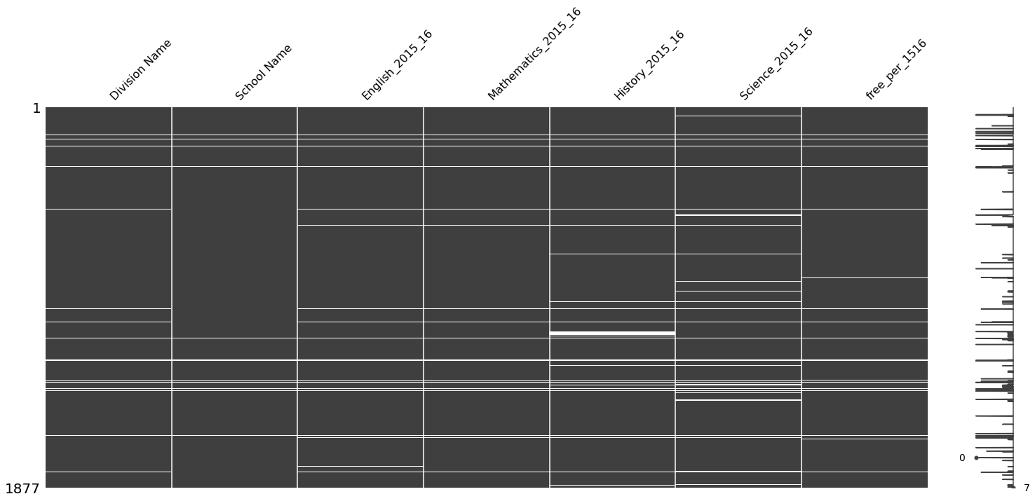
#Output null visualization on combined data frame.
msno.matrix(df)
Division Name School Name English_2015_16 \
count 1822 1831 1813
unique 132 1758 64
top Fairfax County Mountain View Elementary 85
freq 192 6 89
Mathematics_2015_16 History_2015_16 Science_2015_16 free_per_1516
count 1814 1768 1750 1819
unique 62 49 71 1555
top 90 94 83 100.00%
freq 95 99 79 48
Your null count for "df" is:
Null Count Null %
Division Name 55 2.930208
School Name 46 2.450719
English_2015_16 64 3.409696
Mathematics_2015_16 63 3.356420
History_2015_16 109 5.807139
Science_2015_16 127 6.766116
free_per_1516 58 3.090037
<AxesSubplot:>
#Cell 3
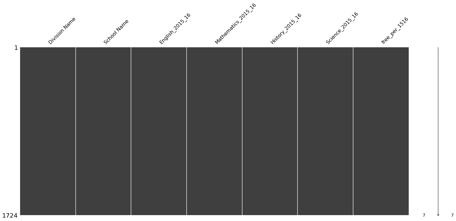
#Drop rows with nulls dependent
df = df.dropna()
#Count nulls again
nullcounter("df")
#Desciribe data frame again.
print(df.describe())
#Visualize nulls again
msno.matrix(df)Your null count for "df" is:
Empty DataFrame
Columns: [Null Count, Null %]
Index: []
Division Name School Name English_2015_16 \
count 1724 1724 1724
unique 132 1662 64
top Fairfax County Mountain View Elementary 85
freq 190 5 84
Mathematics_2015_16 History_2015_16 Science_2015_16 free_per_1516
count 1724 1724 1724 1724
unique 61 49 71 1476
top 90 94 83 100.00%
freq 90 97 79 47
<AxesSubplot:>
#Cell 4
#Check for duplicates on all rows

#Check for duplicates
duplicates = df.duplicated()
print("Duplicate data on all rows combined?")
print(duplicates.unique())
print('\n')

#Check for duplicates on index using duplicated() method, sodee snipped from stackoverflow (Matthew, 2013).
df[df.index.duplicated(keep=False)]

print("Data Types")
df.dtypes
Duplicate data on all rows combined?
[False]
Data Types
Division Name object
School Name object
English_2015_16 object
Mathematics_2015_16 object
History_2015_16 object
Science_2015_16 object
free_per_1516 object
dtype: object
#Cell 5
#Convert scores to numeric then integers
df['English_2015_16'] = pd.to_numeric(df['English_2015_16']).astype(int)
df['Mathematics_2015_16'] = pd.to_numeric(df['Mathematics_2015_16']).astype(int)
df['History_2015_16'] = pd.to_numeric(df['History_2015_16']).astype(int)
df['Science_2015_16'] = pd.to_numeric(df['Science_2015_16']).astype(int)


#remove percentage sign and convert to decimal notation using rstrip and astype.  Code snipped from stackoverflow (Bloom, 2014).
df['free_per_1516'] = df['free_per_1516'].str.rstrip('%').astype('float') / 100.0


#Remove data that is out of bounds in 'free_per_1516'.  Code snipped from stackoverflow (Harikrishnan, 2020).
df.drop(df[df.free_per_1516>1.0].index, inplace=True)
df.drop(df[df.free_per_1516<0.0].index, inplace=True)


#Create a sum of all test scores as 'total_score'.
df['total_score'] = df[["English_2015_16","Mathematics_2015_16", "History_2015_16", "Science_2015_16"]].sum(axis=1)
df.head()


df.free_per_1516.describe()
count 1718.000000
mean 0.402871
std 0.260002
min 0.002800
25% 0.204550
50% 0.372850
75% 0.540700
max 1.000000
Name: free_per_1516, dtype: float64
#Cell 6
#Data nearly cleaned, output visualizations
#Output histogram on free_per_1516
plt.hist(df['free_per_1516'])
plt.title("Histogram {}".format("free_per_1516"))
plt.xlabel("free_per_1516")
plt.ylabel("Count")
plt.show()
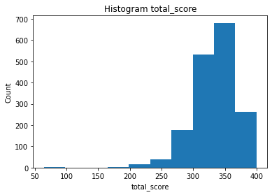
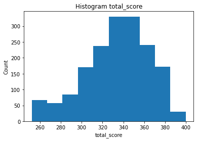
#Output histogram on 'total_score'
plt.hist(df['total_score'])
plt.title("Histogram {}".format("total_score"))
plt.xlabel("total_score")
plt.ylabel("Count")
plt.show()
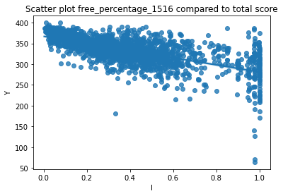
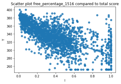
#Output regplot to examine possible relationships
sns.regplot(x = df['free_per_1516'], y = df['total_score'])
plt.title("Scatter plot free_percentage_1516 compared to total score")
plt.xlabel("I")
plt.ylabel("Y")
plt.show()
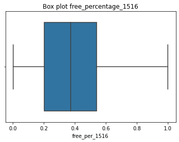
#Output boxplot to examine data characteristics of 'free_per_1516'
sns.boxplot(df['free_per_1516'])
plt.title("Box plot free_percentage_1516")
plt.show()
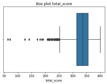
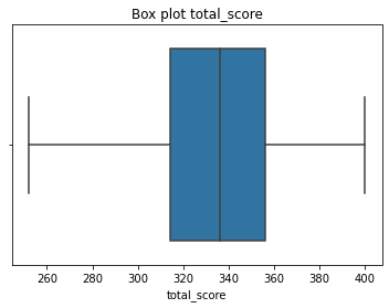
#Output boxplot to examine data characteristics of 'total_score'
sns.boxplot(df['total_score'])
plt.title("Box plot total_score")
plt.show()
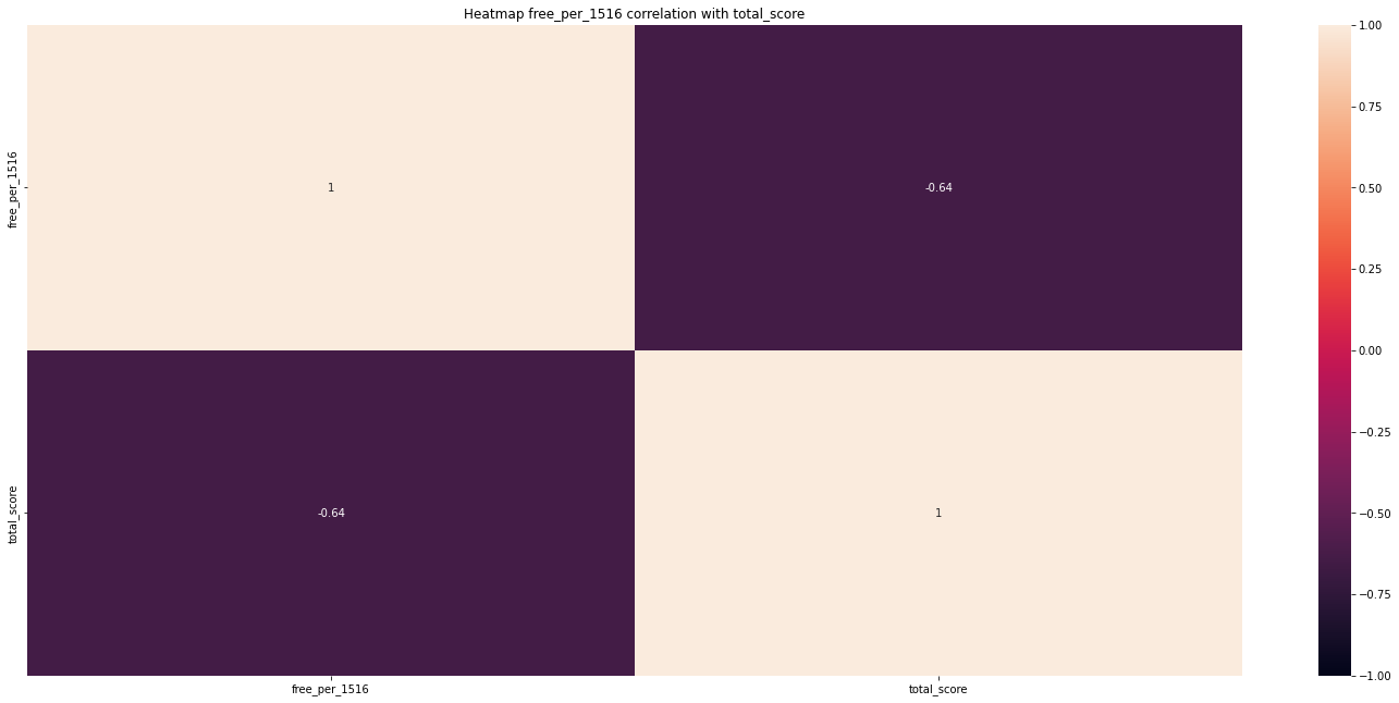
#Output heatmap to examine correlation
plt.figure(figsize=(25, 11))
plt.title("Heatmap free_per_1516 correlation with total_score")
sns.heatmap(df[["free_per_1516","total_score"]].corr(),vmin=-1, vmax=1, annot=True);
#Find median and print
free_lunch_percent_median = df['free_per_1516'].describe().loc[['50%']]
print("Median Percent of 'free_per_1516' is: ", free_lunch_percent_median[0], "\n")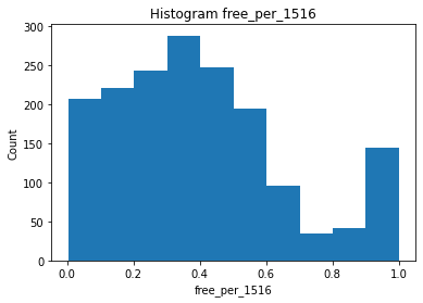
Median Percent of 'free_per_1516' is: 0.37285
#Cell 7
#Capping the data in the skewed distribution "total_score" with 1.5 iqr
#Article mentions treating outliers differently depending on the distribution (Goyal, 2022).

skewed_int_outliers =["total_score"]

#Skewed Distribution Outlier treatment with 1.5iqr
for i in skewed_int_outliers:
    percentile25 = df[i].quantile(0.25)
    percentile75 = df[i].quantile(0.75)
    iqr = percentile75 - percentile25
    upper_limit = percentile75 + 1.5 * iqr
    lower_limit = percentile25 - 1.5 * iqr
    #capping the outliers
    df[i] = np.where(
        df[i]>upper_limit,
        np.rint(math.floor(upper_limit)).astype(int),
        np.where(
            df[i]<lower_limit,
            np.rint(math.ceil(lower_limit)).astype(int),
            df[i]
        )
    )


#Data cleaned, start with visualizations
#Output histogram on free_per_1516
plt.hist(df['free_per_1516'])
plt.title("Histogram {}".format("free_per_1516"))
plt.xlabel("free_per_1516")
plt.ylabel("Count")
plt.show()


#Output histogram on 'total_score'
plt.hist(df['total_score'])
plt.title("Histogram {}".format("total_score"))
plt.xlabel("total_score")
plt.ylabel("Count")
plt.show()


#Output regplot to examine possible relationships
sns.regplot(x = df['free_per_1516'], y = df['total_score'])
plt.title("Scatter plot free_percentage_1516 compared to total score")
plt.xlabel("I")
plt.ylabel("Y")
plt.show()


#Output boxplot to examine data characteristics of 'free_per_1516'
sns.boxplot(df['free_per_1516'])
plt.title("Box plot free_percentage_1516")
plt.show()


#Output boxplot to examine data characteristics of 'total_score'
sns.boxplot(df['total_score'])
plt.title("Box plot total_score")
plt.show()


#Output heatmap to examine correlation
plt.figure(figsize=(25, 11))
plt.title("Heatmap free_per_1516 correlation with total_score")
sns.heatmap(df[["free_per_1516","total_score"]].corr(),vmin=-1, vmax=1, annot=True);


#Find median and print
free_lunch_percent_median = df['free_per_1516'].describe().loc[['50%']]
print("Median Percent of 'free_per_1516' is: ", free_lunch_percent_median[0], "\n")

Median Percent of 'free_per_1516' is: 0.37285

#Cell 8

#Create distinct gropus of student population based on proportion of students who are eligible for free lunch.
#Values below and above can be replaced based on condition (Komali, 2021).

#Split data into 0.372850 (median of cleaned data set)
df.loc[df['free_per_1516'] >= free_lunch_percent_median[0], 'groups'] = 1
df.loc[df['free_per_1516'] < free_lunch_percent_median[0], 'groups'] = 0

df['groups'] = pd.to_numeric(df['groups']).astype(int)
df.groups.describe()

low_percentage_df = df.loc[df['groups'] == 0]
high_percentage_df = df.loc[df['groups'] == 1]


#Export a copy of the cleaned data
df.to_csv("C:\\Users\\will\\Desktop\\Courses\\11 - Capstone - D214\\Task 2\\Data\\cleaned_data.csv", index = False)


#use levene test to check for equality of variance (Bobbit, 2020).
stats.levene(low_percentage_df.total_score, high_percentage_df.total_score, center='median')
LeveneResult(statistic=54.81184644296979, pvalue=2.0681326644527468e-13)
Interpreting the LeveneResult - " Ignore the result. With equal, or nearly equal, sample size (and moderately large samples), the assumption of equal standard deviations is not a crucial assumption. The t test work pretty well even with unequal standard deviations. In other words, the t test is robust to violations of that assumption so long as the sample size isn’t tiny and the sample sizes aren’t far apart. If you want to use ordinary t tests, " (How to Compare Two Means When the Groups Have Different Standard Deviations. - FAQ 1349 - GraphPad, n.d.).
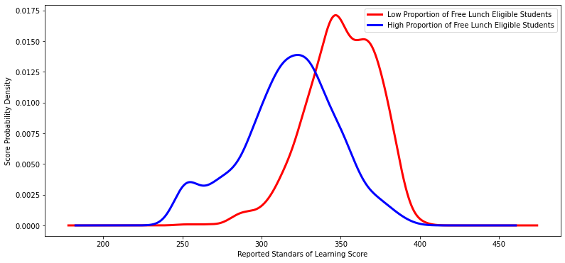
#Cell 9
#Run the t-test
#Code snippet for t-test derived from website (GeeksforGeeks, 2022).
print(stats.ttest_ind(a=low_percentage_df.total_score, b=high_percentage_df.total_score, equal_var=False))

#Plot both population's metrics
low_percentage_df['total_score'].plot(kind='kde', c='red', linewidth=3, figsize=[13,6])
high_percentage_df['total_score'].plot(kind='kde', c='blue', linewidth=3, figsize=[13,6])
# Labels
labels = ['Low Proportion of Free Lunch Eligible Students', 'High Proportion of Free Lunch Eligible Students']
plt.legend(labels)
plt.xlabel('Reported Standars of Learning Score')
plt.ylabel('Score Probability Density')

plt.show()
Ttest_indResult(statistic=25.734340600381046, pvalue=2.5360699249948364e-122)
Original Outcome Complete
#Cell 10
#Make a list of unique divisions
division_list_low = low_percentage_df['Division Name'].unique().tolist()
division_list_high = high_percentage_df['Division Name'].unique().tolist()

print("Count of Divisions with low proportions of students who are eligible for free lunch")
print(len(division_list_low))
print("Count of Divisions with high proportions of students who are eligible for free lunch")
print(len(division_list_high))


#Create a list of divisions that contain schools with high and low proportions of students eligible for free lunch.
#code snippet found online (Chattar, 2021).
divisions_high_and_low_temp = set(division_list_low).intersection(division_list_high)


print("Count of Divisions that have schools with high and low proportions of students eligible for free lunch")
print(len(divisions_high_and_low_temp))

divisions_high_and_low = []
for i in divisions_high_and_low_temp:
    X =low_percentage_df.loc[low_percentage_df['Division Name'] == (i)].total_score
    Y = high_percentage_df.loc[high_percentage_df['Division Name'] == (i)].total_score
    if len(X) > 2 and len(Y) > 2:
        divisions_high_and_low.append(i)

print("Count of Divisions that have more than 2 of each, schools with high proportion of students eligible\
for free lunch, and schools with low proportions.")
print(len(divisions_high_and_low))
Count of Divisions with low proportions of students who are eligible for free lunch
85
Count of Divisions with high proportions of students who are eligible for free lunch
117
Count of Divisions that have schools with high and low proportions of students eligible for free lunch
70
Count of Divisions that have more than 2 of each, schools with high proportion of students eligiblefor free lunch, and schools with low proportions.
32
Ttest_indResult(statistic=6.409940604162604, pvalue=6.681972140013619e-07)
#Cell 11
#Create a selection process with divisions that have a difference in mean test outcomes
divisions_with_low_p_values = []
#To count how many divisions have a < .05 t-score
for i in divisions_high_and_low:
#Geeksforgeeks code snippet(GeeksforGeeks, 2022).
X = low_percentage_df.loc[low_percentage_df['Division Name'] == (i)].total_score
Y = high_percentage_df.loc[high_percentage_df['Division Name'] == (i)].total_score
t,p = stats.ttest_ind(a=X, b=Y, equal_var=False)
if p < .05:
divisions_with_low_p_values.append(i)
print("These divisions have multiple schools with high proportions of students eligible for free lunch and multiple\
schools with low proportions of students eligible for free lunch.")
print("They also show a statistically significant difference in mean test scores.\n")
pprint(divisions_with_low_p_values)
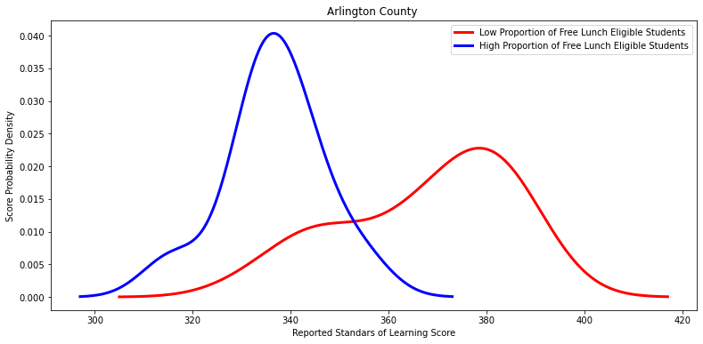
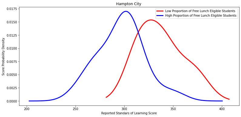
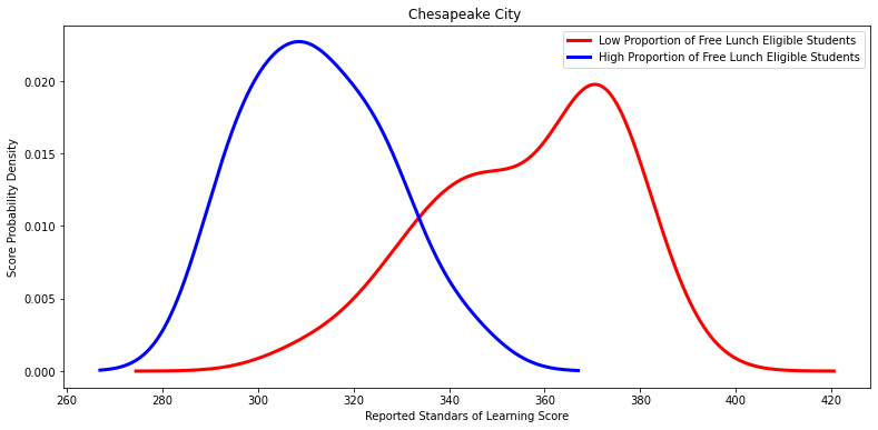
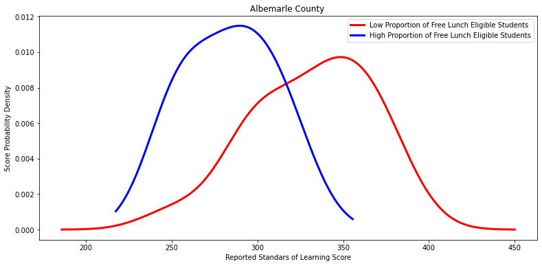
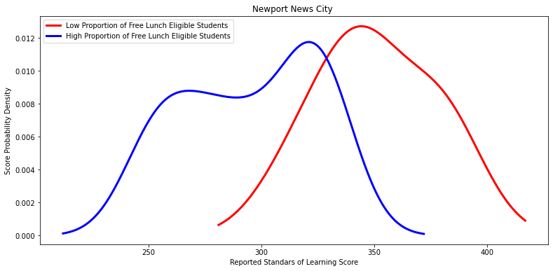
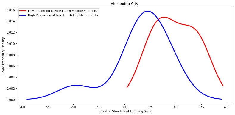
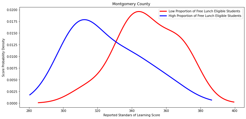
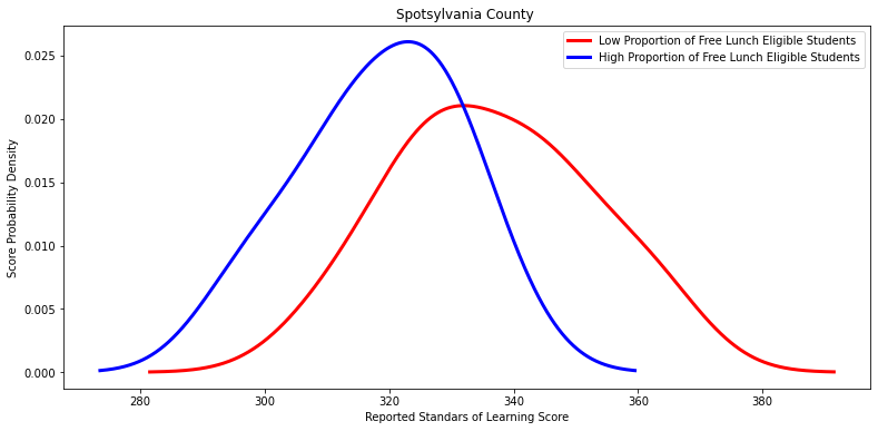
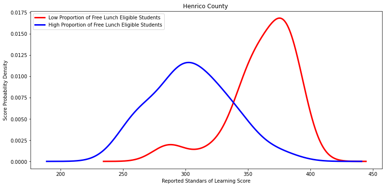
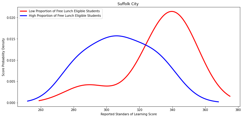
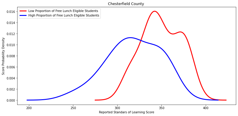
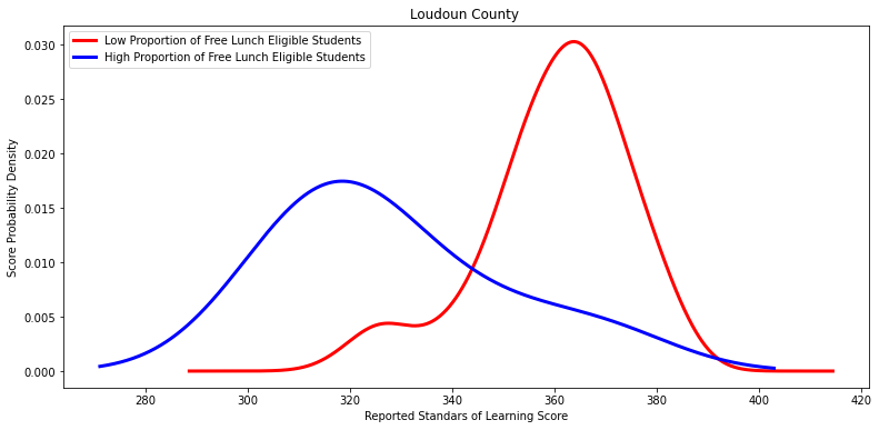
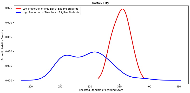
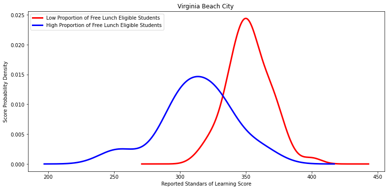
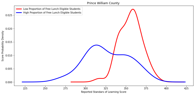
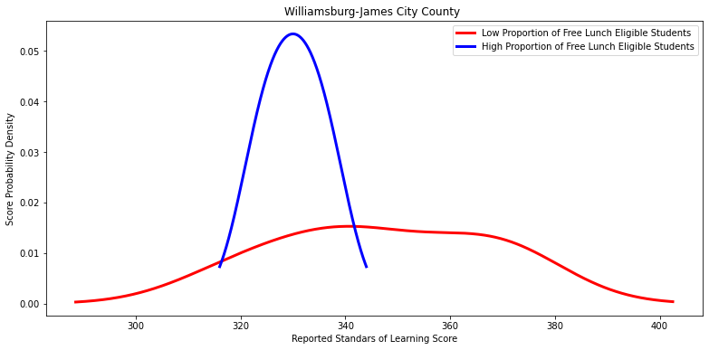
#Visualize density plot on divisions with statistical differences in populations
for i in divisions_with_low_p_values:
X =low_percentage_df.loc[low_percentage_df['Division Name'] == (i)].total_score
Y = high_percentage_df.loc[high_percentage_df['Division Name'] == (i)].total_score
#Run the t-test and output
#Plot both metrics
low_percentage_df.loc[low_percentage_df['Division Name'] == (i)].total_score.plot\
(kind='kde', c='red', linewidth=3, figsize=[13,6])
high_percentage_df.loc[high_percentage_df['Division Name'] == (i)].total_score.plot\
(kind='kde', c='blue', linewidth=3, figsize=[13,6])
# Labels
labels = ['Low Proportion of Free Lunch Eligible Students', 'High Proportion of Free Lunch Eligible Students']
plt.title(i)
plt.legend(labels)
plt.xlabel('Reported Standars of Learning Score')
plt.ylabel('Score Probability Density')
plt.show()
#Code snippet for t-test derived from website (GeeksforGeeks, 2022).
print(stats.ttest_ind(a=X, b=Y, equal_var=False), "\n\n")These divisions have multiple schools with high proportions of students eligible for free lunch and multiple schools with low proportions of students eligible for free lunch.
They also show a statistically significant difference in mean test scores.
['Arlington County ',
'Hampton City ',
'Chesapeake City ',
'Albemarle County ',
'Newport News City ',
'Alexandria City ',
'Montgomery County ',
'Spotsylvania County ',
'Henrico County ',
'Suffolk City ',
'Chesterfield County ',
'Loudoun County ',
'Norfolk City ',
'Virginia Beach City ',
'Prince William County ',
'Williamsburg-James City County ',
'Fairfax County ']
Ttest_indResult(statistic=8.461103427033763, pvalue=4.2564535128111695e-10)
Ttest_indResult(statistic=3.7223282464849152, pvalue=0.0022359663924919103)
Ttest_indResult(statistic=4.806338810130206, pvalue=0.0014819298232501942)
Ttest_indResult(statistic=2.5438908135728764, pvalue=0.027946988309494193)
Ttest_indResult(statistic=2.625164815841848, pvalue=0.023337646472250697)
Ttest_indResult(statistic=3.373751982093548, pvalue=0.0024706357289852967)
Ttest_indResult(statistic=8.196062297626334, pvalue=1.3567694425275851e-11)
Ttest_indResult(statistic=2.4614922901402174, pvalue=0.029589168699507278)
Ttest_indResult(statistic=4.370459142644502, pvalue=0.00011089458080339332)
Ttest_indResult(statistic=4.0471544101064145, pvalue=0.00411407734704421)
Ttest_indResult(statistic=7.659633097156011, pvalue=6.205830981719048e-08)
Ttest_indResult(statistic=6.415834167155425, pvalue=5.255180694823957e-07)
Ttest_indResult(statistic=6.162598621901206, pvalue=1.0118260722466614e-07)
Ttest_indResult(statistic=2.5713849399256987, pvalue=0.02332371134812441)
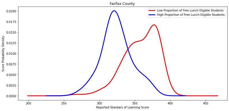
Ttest_indResult(statistic=9.026177677291102, pvalue=3.656434012894371e-14)
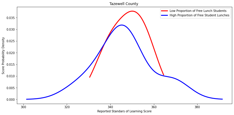
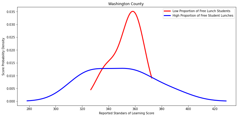
#Cell 12
#Generate list of remaining divisions that didn't have low p-values, but had both types of schools.
#Subtract "divisions_with_low_p_values" from "divisions_high_and_low" using symmetric_difference() method (Hadzhiev, n.d.).
other_divisions = list(set(divisions_high_and_low).symmetric_difference(divisions_with_low_p_values))
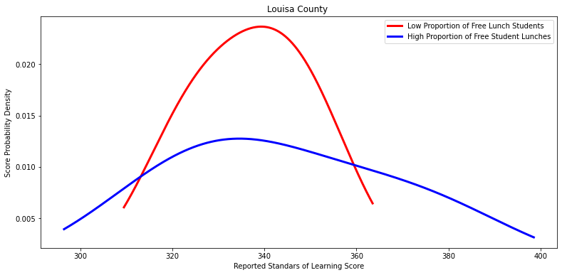
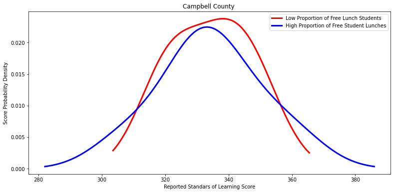
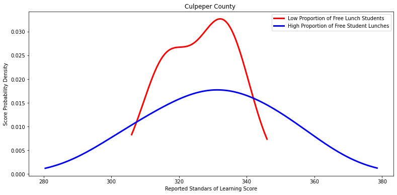
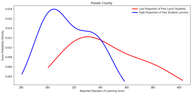
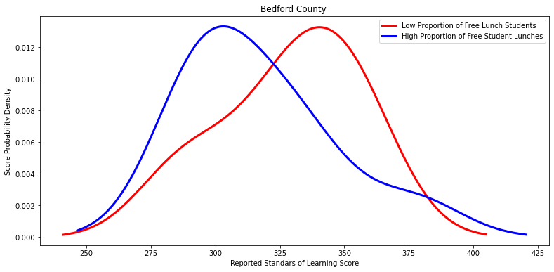
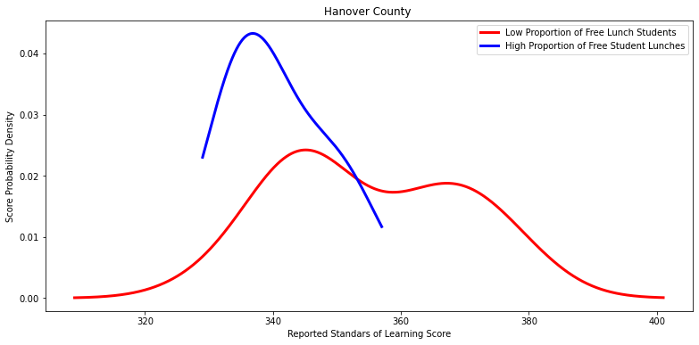
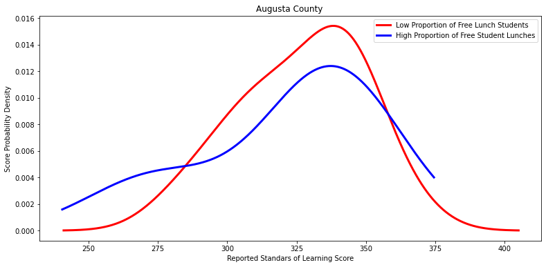
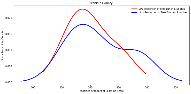
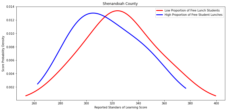
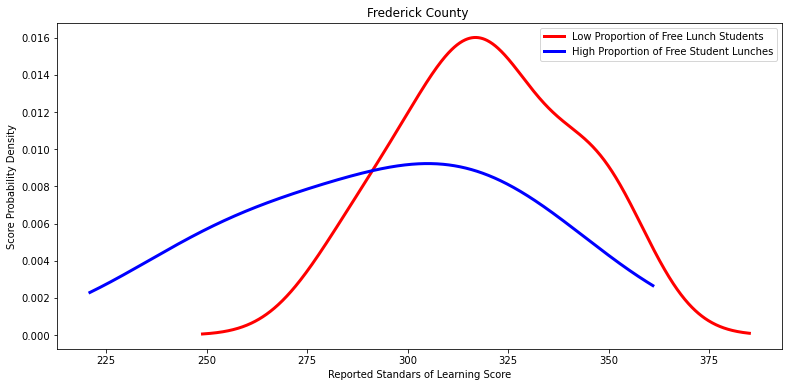
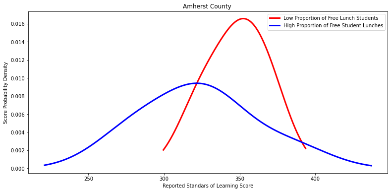
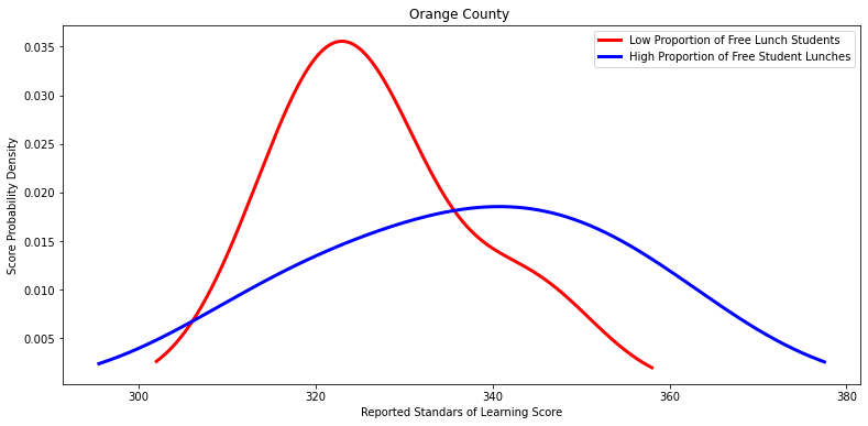
#Visualize density plot on divisions that did not show a statistically significant difference
for i in other_divisions:
X =low_percentage_df.loc[low_percentage_df['Division Name'] == (i)].total_score
Y = high_percentage_df.loc[high_percentage_df['Division Name'] == (i)].total_score
#Plot both metrics
low_percentage_df.loc[low_percentage_df['Division Name'] == (i)].total_score.plot\
(kind='kde', c='red', linewidth=3, figsize=[13,6])
high_percentage_df.loc[high_percentage_df['Division Name'] == (i)].total_score.plot\
(kind='kde', c='blue', linewidth=3, figsize=[13,6])
# Labels
labels = ['Low Proportion of Free Lunch Students', 'High Proportion of Free Student Lunches']
plt.title(i)
plt.legend(labels)
plt.xlabel('Reported Standars of Learning Score')
plt.ylabel('Score Probability Density')
plt.show()
#Code snippet for t-test derived from website (GeeksforGeeks, 2022).
print(stats.ttest_ind(a=X, b=Y, equal_var=False), "\n\n")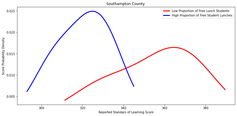
Ttest_indResult(statistic=2.4205691334017856, pvalue=0.08475385838978879)
Ttest_indResult(statistic=0.2570834615381291, pvalue=0.8082157582528549)
Ttest_indResult(statistic=0.6151089286608511, pvalue=0.5499385169889386)
Ttest_indResult(statistic=-0.43228762054052156, pvalue=0.694690937976563)
Ttest_indResult(statistic=0.006819058031850852, pvalue=0.9946954512431896)
Ttest_indResult(statistic=-0.42914107542287455, pvalue=0.6827212468291588)
Ttest_indResult(statistic=1.496028353478178, pvalue=0.23104670043725686)
Ttest_indResult(statistic=0.9439871944160111, pvalue=0.35882922068937606)
Ttest_indResult(statistic=2.4589999935373332, pvalue=0.05995075594533983)
Ttest_indResult(statistic=0.27940572225992494, pvalue=0.794558661937718)
Ttest_indResult(statistic=-0.5999889539606617, pvalue=0.5672948520140612)
Ttest_indResult(statistic=0.5857229902989585, pvalue=0.577275098608178)
Ttest_indResult(statistic=1.2074039981491638, pvalue=0.3369371944307884)
Ttest_indResult(statistic=1.3789234479354537, pvalue=0.2061614549792278)
Ttest_indResult(statistic=-1.0811022683078786, pvalue=0.3315247080127098)
References:
Bloom, G., [GaryMBloom]. (2014, September 4). Convert percent string to float in pandas read_csv. Stack Overflow. https://stackoverflow.com/questions/25669588/convert-percent-string-to-float-in-pandas-read-csv
Bobbit, Z. (2020, July 10). How to Perform Levene’s Test in Python. Statology. https://www.statology.org/levenes-test-python/
Bobbit, Z. (2021, November 6). How to Merge Two Pandas DataFrames on Index. Statology. https://www.statology.org/pandas-merge-on-index/
Chattar, P. (2021, September 2). Find common elements in two lists in python. Java2Blog. https://java2blog.com/find-common-elements-in-two-lists-python/
GeeksforGeeks. (2022, October 17). How to Conduct a Two Sample T Test in Python. https://www.geeksforgeeks.org/how-to-conduct-a-two-sample-t-test-in-python/
Goyal, C. (2022, August 25). Feature Engineering – How to Detect and Remove Outliers (with Python Code). Analytics Vidhya. https://www.analyticsvidhya.com/blog/2021/05/feature-engineering-how-to-detect-and-remove-outliers-with-python-code/
Hadzhiev, B. (n.d.). Remove common elements from two Lists in Python | bobbyhadz. Blog - Bobby Hadz. https://bobbyhadz.com/blog/python-remove-common-elements-from-two-lists
Harikrishnan, R., [Harikrishnan R]. (2020, January 26). Dropping rows with values outside of boundaries. Stack Overflow. https://stackoverflow.com/questions/59914605/dropping-rows-with-values-outside-of-boundaries
How to compare two means when the groups have different standard deviations. - FAQ 1349 - GraphPad. (n.d.). GraphPad by Dotmatics. https://www.graphpad.com/support/faq/how-to-compare-two-means-when-the-groups-have-different-standard-deviations/
Inada, I. (Ed.). (n.d.). Replacing values with NaNs in Pandas DataFrame. https://www.skytowner.com/explore/replacing_values_with_nans_in_pandas_dataframe
Komali. (2021, December 27). Pandas Replace Values based on Condition. Spark by {Examples}. https://sparkbyexamples.com/pandas/pandas-replace-values-based-on-condition/
Matthew. (2013, November 25). Pandas: Get duplicated indexes. Stack Overflow. https://stackoverflow.com/questions/20199129/pandas-get-duplicated-indexes